Fast Face Detector
Project on GitHub: IggyShone/fast_face_detector
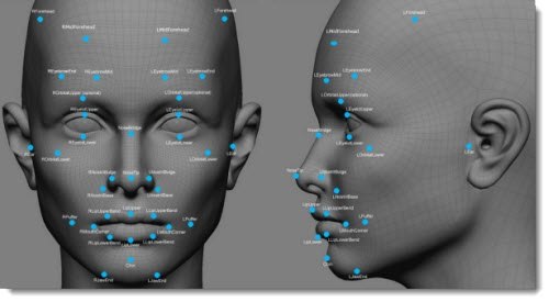
Face detection, a sub problem of object detection , is a challenging task due to the fact that faces may appear in various pose, scale, facial expression, occlusion, and lighting settings. One of the simplest and common ways to perform an object detection in the world of deep neural networks is a sliding window approach where an image is scanned sequentially, by running a network on it, inspecting each fixed size window at a time. Unfortunately, despite giving (if trained correctly) promising accuracy ,this routine is costly and therefore greatly degenerates a given detector speed. A better solution would be to transform a given network into a fully-convolutional network by converting fully-connected layers to convolution layers. The reason therefore lay in the fact that convolutional outputs are shared between multiple windows.
The output of a fully convolutional network (FCN) on a given image is a probability map for the existence of the object in each window. The size of the window is the network input size while the stride between each window is decided by the amount of down sampling the network performs.
For instance: consider activating a fully convolutional network with input size of 227 and stride of 32 over an input image of size 451 × 451. The equation for output map:
output = (input − network_input_size)/stride + 1 = (451 − 227)/32 + 1 = 8
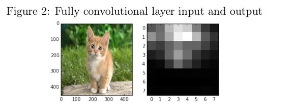
Each cell (i, j) in the heat-map contains the probability for an object (a face in our case) to exist in a window with bottom left point (32i, 32j) of spatial size 32 × 32.
For more detail explanation on convolutional neural networks and FCN in general and the transformation between those two in detail please refer to: CS231n Convolutional Neural Networks for Visual Recognition
Step 1: face / non-face classifier
When inspecting a specific window at some size we’d need to binary classify it deciding weather the pixels in that window constitutes a face or not.
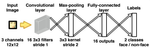
A simple shallow convolutional network would do the job. The network receives as input a patch of size 12 × 12 from a RGB image - and classifies it as either face or non-face. As positive samples we’d use AFLW faces while for the negative we’d crop random patches from the PASCAL data-set
System Scheme
Model
local model = nn.Sequential();
-- input 3x12x12
model:add(nn.SpatialConvolution(3, 16, 3, 3))
-- outputs 16x10x10
model:add(nn.SpatialMaxPooling(3, 3, 2, 2))
model:add(nn.ReLU())
-- outputs 16x4x4
model:add(nn.SpatialConvolution(16, 16, 4, 4))
model:add(nn.ReLU())
-- outputs 16x1x1
model:add(nn.SpatialConvolution(16, 2, 1, 1))
-- outputs 2x1x1
model:add(nn.SpatialSoftMax())
-- handling with diminishing gradients
model:add(nn.AddConstant(0.000000001))
model:add(nn.Log())
Definitions
----------------
-- LOSS FUNCTION
----------------
local criterion = nn.CrossEntropyCriterion()

---------------
-- TRAINING
---------------
local parameters, gradParameters = model:getParameters()

------------------------------
-- Closure with mini-batches
------------------------------
local counter = 0
local feval = function(x)
	if x ~= parameters then
		parameters:copy(x)
	end
	local start_index = counter * opt.batch_size + 1
	local end_index = math.min(opt.train_size, (counter + 1) *
 	opt.batch_size)
	if end_index == opt.train_size then
		counter = 0
	else
		counter = counter + 1
	end
	local batch_inputs = data[{{start_index, end_index}, {}}]
	local batch_targets = labels[{{start_index, end_index}}]
	gradParameters:zero()

	-- 1. compute outputs (log probabilities) for data point
	local batch_outputs = model:forward(batch_inputs)
	-- 2. compute the loss of these outputs, measured against
		the true labels in batch_target
	local batch_loss = criterion:forward(batch_outputs,
	batch_targets)
	-- 3. compute the derivative of the loss wrt the outputs of
	the model
	local loss_doutput = criterion:backward(batch_outputs,
	batch_targets)
	-- 4. use gradients to update weights
	model:backward(batch_inputs, loss_doutput)

	return batch_loss, gradParameters
end
Training is done on mini-batches while minimizing a cross entropy loss function.
Optimization
-- OPTIMIZE
-----------
local train_losses = {}
local test_losses = {}

-- # epoch tracker
epoch = epoch or 1

for i = 1,opt.epochs do

	trimModel(model)

	-- shuffle at each epoch
	local shuffled_indexes =
	torch.randperm(data:size(1)):long()
	data = data:index(1,shuffled_indexes)
	labels = labels:index(1,shuffled_indexes)

	local train_loss_per_epoch = 0
	-- do one epoch
	print('==> doing epoch on training data:')
	print("==> online epoch # " .. epoch .. ' [batchSize = ' ..
 	opt.batch_size .. ']')

	for t = 1,opt.train_size,opt.batch_size do
		if opt.optimization == 'sgd' then
			_, minibatch_loss  = optim.sgd(feval, parameters,
			optimState)
			print('mini_loss: '..minibatch_loss[1])
			train_loss_per_epoch = train_loss_per_epoch +
			minibatch_loss[1]
		end
	end
	-- update train_losses average among all the mini batches
	train_losses[#train_losses + 1] = train_loss_per_epoch /
	(math.ceil(opt.train_size/opt.batch_size)-1)

	-------------
	-- TEST
	-------------
	trimModel(model)

	local test_data = data[{{opt.train_size+1, data:size(1)},
	{}}]
	local test_labels = labels[{{opt.train_size+1,
	data:size(1)}}]

	local output_test = model:forward(test_data)
	local err = criterion:forward(output_test, test_labels)

	test_losses[#test_losses + 1] = err
	print('test error ' .. err)

	logger:add{train_losses[#train_losses],
	test_losses[#test_losses]}

end
We plot the cost function value for test and train after each epoch and monitor the classification error. Also compactly saving the model at end.
--------------------------------------------------------
--  PLOTTING TESTING/TRAINING LOSS/CLASSIFICATION ERRORS
--------------------------------------------------------
gnuplot.pdffigure('loss_12net.pdf')
gnuplot.plot({'train loss',torch.range(1, #train_losses),torch.Tensor(train_losses)},
	{'test loss',torch.Tensor(test_losses)})
gnuplot.title('loss per epoch')
gnuplot.figure()

---------------
-- SAVING MODEL
---------------
local fmodel = model : clone (): float ()
for i =1 ,# fmodel.modules do
	local layer = fmodel : get ( i )
	if layer.output ~= nil then
		layer.output = layer.output.new ()
	end
	if layer.gradInput ~= nil then
		layer.gradInput = layer.gradInput.new ()
	end
end

torch.save('model_12net.net', fmodel)
Results
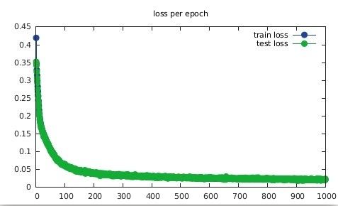
We see that generalization succeeded (blue curve is hidden by the green one) with a classification error of 0.0145836.
Step 2: Repeat step 1 only this time with 24×24 and 48×48 sized windows.
The difference from the previous step is the source of the negative labels. For the 24×24 net, each window classified as positive in the 12×12 net would now serve as a negative example. This method is known as negative boostraping. Apply same to the 48×48 net w.r.t 24×24.
- So far We have built three stand-alone convolutional networks which constitutes the main building blocks of the face detector we just about to describe its pipeline.
Step 3: Detector pipeline
Given a test image, we’d want quickly to perform a dense scan to reject as much as possible of the detection windows though maintaining a high recall (eliminate many false negatives but keep many true positives). The 12×12 net is fast in that sense due to its relatively shallowness.
There is a problem however. Practically a face in an image could come up with different sizes (not necessarily fit to the fixed convolution nets input size). Thus we must scan the image across different scales. In computer vision this is called an image pyramid.

If the face size is X, the test image is first built into image pyramid to cover faces at different scales and each level in the image pyramid is re-sized by 12X as the input image for the 12×12 net.
Creating image pyramid
local smallestImgDim = 100000
scales = {} -- list of scales
-- 20 is a system hyper param dependable on our prior knowledge
-- on face sizes. Acurracy vs performance tradeoff.
for k =1 ,20 do
	local scale = 12/( smallestImgDim /20+ smallestImgDim *(k
		-1)/20)
	if scale * smallestImgDim < 12 then break end
		table.insert (scales , scale )
end

-- create pyramid packer and unpacker. scales is a table with
-- all the scales you with to check.
local unpacker = nn.PyramidUnPacker(model)
local packer = nn.PyramidPacker(model, scales)
Therefore the result of that dense scan across different scales (via the 12×12 net) is a map of confidence scores for faces detections.
-- dense scan across different scales
local multiscale  = model_12net:forward(pyramid)
	-- unpack pyramid , distributions will be table of tensors
	local distributions = unpacker_12:forward(multiscale ,
		coordinates)
	local val, ind, res = 0
	local detections_12net = {}

	-- iterate on the map of confidence scores
	-- determining a face if p>threshold
	for j = 1,#distributions do
		local boxes = {}
		distributions[j]:apply(math.exp)
		vals, ind = torch.max(distributions[j],1)
		ind_data = torch.data(ind)
		--collect pos candidates (with threshold p>0.5)
		local size = vals[1]:size(2)
		for t = 1,ind:nElement()-1 do
			x_map = math.max(t%size,1)
			y_map = math.ceil(t/size)
			--converting to orig. sample coordinate
			x = math.max((x_map-1)*2 ,1)
			y = math.max((y_map-1)*2 ,1)

			if ind[1][y_map][x_map] == 1 then
				--prob. for a face
				table.insert(boxes, {x,y,x+11,y+11,vals[1]
				[y_map][x_map]})
			end
		end
A side effect due to the many small windows involved could be an overflow of positive overlapped detection. Non-maximum suppression (NMS) is applied to eliminate highly overlapped detection windows.
local pos_suspects_boxes = torch.Tensor(boxes)
		local nms_chosen_suspects = nms(pos_suspects_boxes, 0.5)

		if #nms_chosen_suspects:size() ~= 0 then
			pos_suspects_boxes =
			pos_suspects_boxes:index(1,nms_chosen_suspects)
The remaining detection windows are cropped out and resized into 24×24 images.
for p = 1,pos_suspects_boxes:size(1) do
				--scalling up suspected box to orig size image
				sus = torch.div(pos_suspects_boxes[p],scales[j])
				sus:apply(math.floor)
				croppedDetection = image.crop(img, sus[1],
					sus[2], sus[3], sus[4])
				croppedDetection = image.scale(croppedDetection,
					24, 24)
				table.insert(detections_12net,
				{croppedDetection:resize(1,3,24,24), sus[1],
					sus[2], sus[3], sus[4]})
			end
		end
	end
Then serve as input images for the 24×24 to further reject many of the remaining detection windows.
---- Use 24 net to run on each 12 net detection ----
	local detections_24net = {}
	for d = 1,#detections_12net do
		local dist = model_24net:forward(detections_12net[d][1])
		if math.exp(dist[1][1][1][1]) > math.exp(dist[1][2][1]
			[1]) then
			--image.scale(croppedDetection, 24, 24)
			table.insert(detections_24net,{detections_12net[d]
			[2], detections_12net[d][3],
					detections_12net[d][4], detections_12net[d]
			[5], math.exp(dist[1][1][1][1])})
		end
	end
Same as before, the positive detection windows are applied with NMS to further reduce the number of detection windows.
if #detections_24net ~= 0 then
		local pos_suspects_boxes =
		torch.Tensor(detections_24net)
		local nms_chosen_suspects = nms(pos_suspects_boxes, 0.5)

		if #nms_chosen_suspects:size() ~= 0 then
			pos_suspects_boxes =
			pos_suspects_boxes:index(1,nms_chosen_suspects)
		end

		for n=1, pos_suspects_boxes:size(1) do
			sus = pos_suspects_boxes[n]
			table.insert(detections,sus)
		end
	end
Now repeat Step 3 but change everywhere from 12×12 to 24×24 and 24×24 to 48×48.
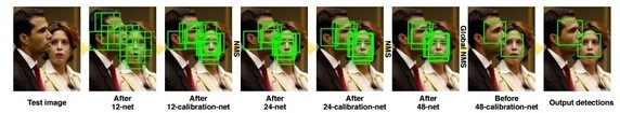
The overall process could be depicted as:
Evaluation
To evaluate the detector we’d use the Face Detection Data Set and Benchmark. We’d need to save the detections in the elliptical format described here.
--find circles (simple ellipse) enclosing
--each bounding box and report detections
	for d = 1,#detections do
		box = detections[d]
		radius = 0.5*math.sqrt(math.pow((box[3] -
			box[1]),2)+math.pow((box[4] - box[2]),2))
		centerX = box[1] + math.floor((box[3] - box[1])/2)
		centerY = box[2] + math.floor((box[4] - box[2])/2)
		-- write detectiodetections_24netn in ellipse format
		io.write(radius ..' '.. radius ..' '.. 0 ..' '.. centerX
		..' '.. centerY ..' '.. 1)
		io.write("\n")
	end
After running the evaluator, the reported recall is 0.924272 with an average running speed of 27ms per image without code optimization (on a G-force gtx 980 ti GPU). The precision wasn’t so good though. I suspect the reason is due to the format conversion loss between the bounding box and the ellipse. However, solving that issue and then plotting the precision-recall curve comparing to other leading face detector curves would be the correct way to proceed.
I would give the reader a chance to experiment that and report the results if he may (:You are welcome to leave any comments and/or questions which I promise to respond as soon as I can.
Email: igor@deep-solutions.net
Deep Solutions wishes you a great deep day!